If you work with electrical systems long enough, you will hear a familiar complaint. “We reduced our electricity use, but the bill did not drop much.” In most cases, the explanation is not mysterious. It is a mismatch between what the person improved and what the tariff charges heavily for. Utilities usually bill you for two different things. One is energy, measured in kilowatt-hours (kWh). The other is demand, measured in kilowatts (kW), or sometimes kilovolt-amperes (kVA). Energy is the total amount used over time. Demand is the highest rate of use during a billing period, based on a defined averaging window. These two are related, but they are not the same. You can reduce one without reducing the other.
I will walk through the definitions, show how meters actually compute demand, and explain the common misunderstandings I see from students and working engineers alike. I will also show practical ways to reduce both charges without guessing.
Start with the units
What is kW vs kWh? Energy is measured in kWh. A kWh is not a “kilowatt per hour.” It is kilowatts multiplied by hours. If you run a 2 kW heater for 3 hours, you use 6 kWh. That is energy.
Demand is measured in kW. A kW is power. It is the rate at which energy is being used at a given time. Utilities often bill demand as the maximum average kW over a short interval. Common intervals are 15 minutes or 30 minutes. The peak interval for the month becomes your billing demand.
When you keep the units straight, the rest becomes easier.
The basic relationship is:
kWh = average kW x hours
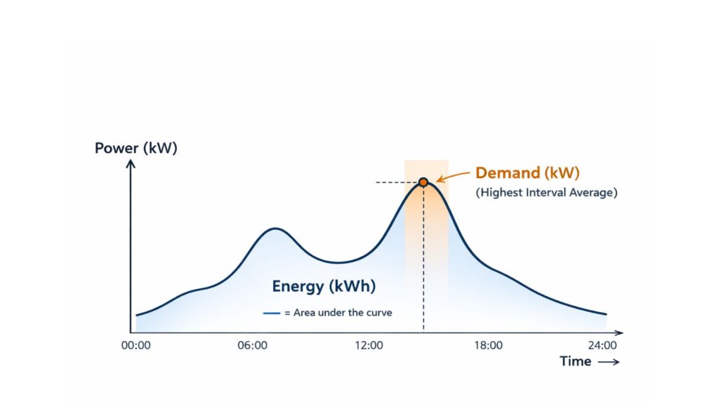
That is why energy is often called “area under the power curve.” Demand is not the area. Demand is the peak level the curve reaches, based on the averaging rule.
A simple mental model that works
Think of electricity like water in a tank.
Energy, kWh, is like the total volume of water you used over a month. Demand, kW, is like the highest flow rate you need at any time. Even if your total water use drops, you can still have one moment where you open many taps at once. The plumbing system must be sized for that moment. Demand charges are the electrical version of paying for the size of the pipe.
That is why demand charges exist. The utility has to build generation, transmission, and distribution capacity that can serve your peak, not just your average.
Why the meter can show kW demand even if you “only measure kWh.”
Modern meters record energy in short time slices. From those slices, the meter calculates interval demand. Conceptually, it does this:

Let’s make that real with a 15-minute interval. Fifteen minutes is 0.25 hours.
If your facility uses 10 kWh during one 15-minute interval, the average power in that interval is:
kw = 10 / 0.25 = 40 kW
The meter repeats that calculation for every interval in the month. The highest interval average becomes your demand for billing, unless your tariff defines a more complex rule such as time-of-use demand or ratchets. The important point is that demand is derived from energy data. It is not magic. It is just energy per interval, converted back into average power.
Worked example: how energy savings can look disappointing on the bill
Consider a small commercial site.
Monthly energy use is 50,000 kWh. Billing demand is 120 kW. The tariff has an energy charge of $0.12 per kWh and a demand charge of $15 per kW. There is also a fixed customer charge of $200.
Energy charge is:
50,000 × 0.12 = $6,000
Demand charge is:
120 × 15 = $1,800
Fixed charge is $200.
The total bill is $8,000.
Now, suppose you improve lighting and reduce energy by 10%. Energy becomes 45,000 kWh. Your energy charge becomes $5,400. You saved $600. That is a real savings.
If your peak demand is still 120 kW, your demand charge stays $1,800. Your fixed charge stays $200. The new total bill is $7,400.
Many people expected a much larger drop because they focused on “we used less electricity.” They did use less energy. But the demand portion did not move. In this example, demand is over 22% of the total bill. In some industrial tariffs, demand can dominate the bill. If demand stays high, the bill stays high.
This is not a reason to avoid energy efficiency. It is a reason to match your projects to your tariff.
The misunderstandings I see most often
Misunderstanding 1: “Demand is the instantaneous peak.”
In most billing tariffs, demand is not a split-second spike. It is an average over a fixed interval. That interval is usually 15 minutes, 30 minutes, or 60 minutes. Utilities publish the interval length in the tariff or billing terms.
This matters for motor starting and inrush. A motor may draw a high current for a few cycles during start. That moment is real. It affects voltage dip and equipment stress. But it may not move demand billing much because it does not last long.
What does move billed demand is the load that lasts long enough inside the interval window. A chiller running hard for 20 minutes. Several compressors start and then run together. Electric heaters are warming up. A production line ramping to full output.
As an engineer, I usually tell people to focus on what is operating during the entire peak interval. That is the demand driver.
Misunderstanding 2: “If I cut kWh, demand must drop too.”
Sometimes it does. Often it does not.
If your project reduces load evenly across the day, the average kW drops, and the kWh drops. But if your peak is caused by specific coincident loads, the peak may not change. Lighting retrofits are a common example. They reduce kWh significantly. They also reduce kW. But your peak might still be set by HVAC, refrigeration, process heating, or air compressors. If those dominate the peak, lighting improvements will not change demand much.
The engineering way to check is simple. Identify the peak demand interval. List the major loads operating in that window. If the retrofit does not touch those loads, demand will not move.
Misunderstanding 3: “It was only one bad day. Why am I paying for it all month?”
Many tariffs set billing demand as the single highest interval in the entire billing period. One unusual day can set the demand for the month. This often happens on Monday mornings, after shutdowns, or after maintenance. Everything starts at once. Controls are not sequenced. Operators turn on multiple systems at the same time. The site hits a high peak that lasts 15 to 30 minutes. The rest of the month might be calmer. The bill still reflects the worst interval.
This is why sequencing and operational discipline can produce fast savings. Sometimes you do not need new equipment. You need a better start-up procedure.
Misunderstanding 4: “We shut down nights and weekends. Demand should be low.”
Shutdowns are great for energy. They reduce operating hours. They reduce kWh. But demand is set by the highest interval. If the highest interval occurs during weekday ramp-up, shutdowns do not help demand.
I see this in warehouses and offices. They run less at night. Energy drops. Demand still spikes at the morning start when HVAC, fans, and equipment all start together. If the morning ramp is not controlled, demand remains high.
Misunderstanding 5: “Our bill uses kW, so power factor does not matter.”
Sometimes this is true. Sometimes it is very false.
Some tariffs bill demand in kVA instead of kW. Some add penalties or adjustments when the power factor is low. If demand is billed in kVA, then the power factor directly affects demand cost.
The relationship is:
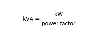
If you have a 120 kW load at 0.80 power factor, kVA is:
120 / 0.80 = 150 kVA
That is a 25% increase. If the demand rate is applied to kVA, your billed demand becomes much higher even though the real power did not change.
For professionals, the key is to read the tariff line item. Does it say kW demand, kVA demand, or does it reference a minimum power factor with penalties? If it is kVA demand, correcting the power factor can reduce demand charges. You still must do it properly. Capacitor sizing, switching steps, resonance risk, and harmonics matter.
Misunderstanding 6: “We reduced demand this month, but the billed demand is still high.”
This is often a ratchet clause.
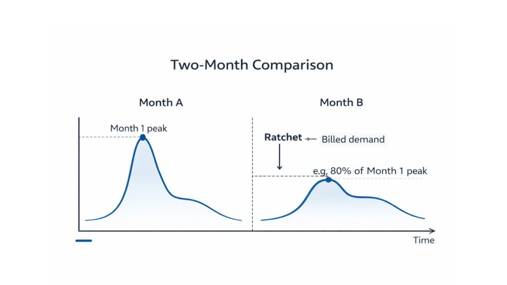
A ratchet is a rule that sets billing demand as the greater of the current month peak and some fraction of a prior peak, often from the last 11 or 12 months. A common structure is 80% to 90% of the highest demand in the past year. Not all utilities use it, but many do for certain customer classes. The logic is that the utility built capacity for your historical peak. Even if you drop demand for one month, the system must still be ready for your return to high demand. The ratchet reduces volatility. From a planning standpoint, this means one extreme peak can raise your bills for many months. It also means demand management is not just a monthly tactic. It is a long game.
Time-of-use demand. Another source of confusion.
Many people understand time-of-use energy rates. Off-peak kWh is cheaper. Peak kWh is more expensive.
Time-of-use demand adds another layer. The utility may charge demand based on the maximum kW during specific peak hours, not the whole day. Some tariffs also charge separate demand values for peak and off-peak periods.
This is why a facility can have a modest overall peak, but a very expensive peak if it occurs during the defined peak window. It also explains why shifting the load by a couple of hours can reduce demand charges even if total energy stays similar.
For students, the takeaway is this. Always ask, “Peak demand during what time window?” The answer changes the strategy.
How to diagnose your demand driver using interval data
If you want to stop guessing, you need interval data. Many utilities provide it. Some meters can output it through a portal. The goal is to find what caused the highest interval.
Here is the method I use in audits.
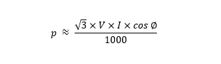
First, locate the billing demand value and the interval length. The bill often shows “kW demand” and the date and time of the peak. If it does not, request interval data. Second, find the top five highest intervals. Do not look only at the highest one. The top few intervals show patterns. You often see the same time of day repeated. Third, cross-check operations. What was running then? If you do not have submetering, talk to the operators. Check BMS trends. Check compressor logs. Check chiller staging data. Check production schedules. The point is to tie the peak interval to actual equipment states. Fourth, do a quick sanity check. If your peak is 120 kW, ask what equipment could plausibly produce that. For three-phase systems, you can estimate current using:
Practical ways to reduce energy charges and demand charges
Energy reduction is usually about efficiency and operating hours. Demand reduction is usually about coincidence and control. Some projects do both. Many do only one. You want to pick the right lever.
Energy reduction projects include lighting retrofits, motor efficiency upgrades, reducing compressed air leaks, improving insulation, and optimizing schedules. These reduce kWh because they reduce the average load or run time.
Demand reduction projects focus on peak intervals. The most common wins come from sequencing. Do not start all large loads at once. Add delays and interlocks. Stage compressors. Prevent simultaneous electric heating and cooling. Limit chiller starts. Use soft starters or VFDs where it reduces sustained kW in the interval. VFDs help most when they reduce real power during operation, not just starting current.
Demand control systems can also shed noncritical loads when demand approaches a threshold. This is common in commercial buildings. The system watches real-time demand and temporarily turns off loads like electric reheats, some HVAC stages, or noncritical pumps. In industrial plants, the same idea applies, but you must protect process quality.
Storage can play a role, too. Thermal storage shifts cooling load. Batteries can shave short peaks. Economics depend on the demand rate, the peak duration, and how often peaks occur.
If your tariff bills kVA demand, power factor correction can reduce the billed demand. But do it carefully. Check harmonic distortion. Check resonance risks. Use staged capacitors and proper controls. In some facilities, active harmonic filters are a better solution because they improve power factor and reduce harmonics.
A short example of demand shaving by sequencing
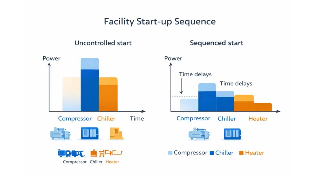
Assume a facility has three large loads that often start together at 8:00 AM.
A compressor draws 35 kW when running. A chiller draws 50 kW at morning pull-down. A process heater draws 40 kW during warm-up. If all three run together in the same 15-minute interval, the site can hit about 125 kW. That might set demand.
If you delay the heater warm-up by 20 minutes, the chiller can complete the hardest part of pull-down before the heater starts. If the compressor is staged properly, it may cycle less aggressively. The peak interval might drop from 125 kW to, say, 95 kW. That is a 30 kW reduction.
If the demand charge is $15 per kW, the monthly demand savings are:
30 × 15 = $450 per month
That can be achieved with controls and procedure changes. This is why demand management is often one of the fastest paybacks, especially in commercial and light industrial sites.
What to teach a student. What to tell a manager.
If I am teaching a student, I emphasize definitions and units. kWh is energy. kW is power. Demand is the highest interval average. Then I give them a plot. Power versus time. The area is kWh. The peak is in demand.
If I am talking to a manager, I translate it into cost levers. kWh projects reduce consumption. Demand projects reduce peaks. The bill is not one knob. It has at least two knobs.
If you want savings to match expectations, you must align the project with the tariff structure.
Common questions I get in the field
People often ask whether solar reduces demand charges. The honest answer is “it depends.” Solar reduces daytime kW when it is producing. If your peak occurs in late afternoon or evening, solar may not help. If your peak occurs during midday cooling, solar can help a lot. You need the interval data to know.
Another frequent question is whether a brief motor start can set demand. Usually no. It can contribute, but only if it meaningfully increases energy within the demand interval. If the motor starts and then runs at high load for the rest of the interval, then yes, it can set demand. The motor start itself is not the main issue. The sustained operation is.
Where a calculator helps
This topic pairs well with a few simple tools.
One is a kW to kWh calculator. You enter the average kW and hours. It gives kWh. This helps students stop confusing power and energy.
Another is a kW and power factor to kVA calculator. This matters when demand is billed in kVA or when you are evaluating power factor correction.
A third is a demand charge estimator. You enter the demand rate and peak kW. It gives the demand charge. If you also have interval data, you can model “what if” scenarios. You can test how much savings you get by shaving 5 kW, 10 kW, or 20 kW.
References and verification notes
For billing details, the source of truth is always the utility tariff or rate schedule for your customer class. It defines interval length, time-of-use windows, ratchets, kW versus kVA billing, and power factor terms.
For engineering fundamentals, standard power and energy relationships are covered in electrical machines and power systems textbooks, as well as utility “how to read your bill” guides. I recommend verifying your specific situation against the tariff language and your meter interval data.
Verification note: The examples above use standard definitions of kW, kWh, interval demand, and basic three-phase power relationships. Real bills can include additional riders, taxes, fuel adjustments, and minimum charges, so the exact dollar outcomes depend on your tariff.